Stop measuring the ocean. Measure the monsoon.
ENSO tells you the odds for the season. It cannot tell you what the monsoon trough will do next week. VIMI decomposes the Indian Summer Monsoon into its seven semi-permanent features and measures each one directly, on operational model output, out to 16 days.
↓ Download full paper (PDF) Worked example — July 2026 →1. The problem VIMI is built for
The Indian Summer Monsoon delivers 70–80% of India's annual rainfall. Its year-to-year swings are usually explained through the El Niño–Southern Oscillation (ENSO), the Indian Ocean Dipole (IOD) and the Madden–Julian Oscillation (MJO). Those are genuinely useful — for the season.
But they share a limitation that is easy to state and hard to work around:
"A critical epistemological limitation of ENSO, IOD, and MJO as monsoon diagnostic tools is that they represent boundary condition drivers rather than direct atmospheric manifestations of the monsoon circulation. Their influence is transmitted through complex teleconnection pathways over weeks to months, is modulated by multiple competing forcings, and carries inherently probabilistic rather than deterministic predictive value. An anomalously strong El Niño does not guarantee monsoon failure."
A sea surface temperature anomaly in the equatorial Pacific is not a measurement of the Indian monsoon. It is a measurement of something that influences it, 12,000 km away, on a timescale of months. Ask it what the monsoon trough over Madhya Pradesh will do in the second week of July and it has nothing to say.
The existing dynamical monsoon indices — Webster-Yang (WYI), Wang-Fan (WFI), Goswami (MHI) — do measure the atmosphere, but each condenses the circulation into a single scalar. When the WYI goes negative, the index alone cannot tell you whether the Somali Jet failed, the monsoon trough shifted to the foothills, the Tibetan Anticyclone weakened, or several of these happened at once. For operational forecasting, that attribution ambiguity is the whole problem.
VIMI's two design choices. First, decompose the monsoon into seven independently measured semi-permanent features rather than one scalar — so an anomaly can be attributed to a specific physical feature. Second, run it on operational GFS output rather than reanalysis only — so it produces a 16-day forward outlook of monsoon phase, not just a diagnosis after the fact.
2. The seven components
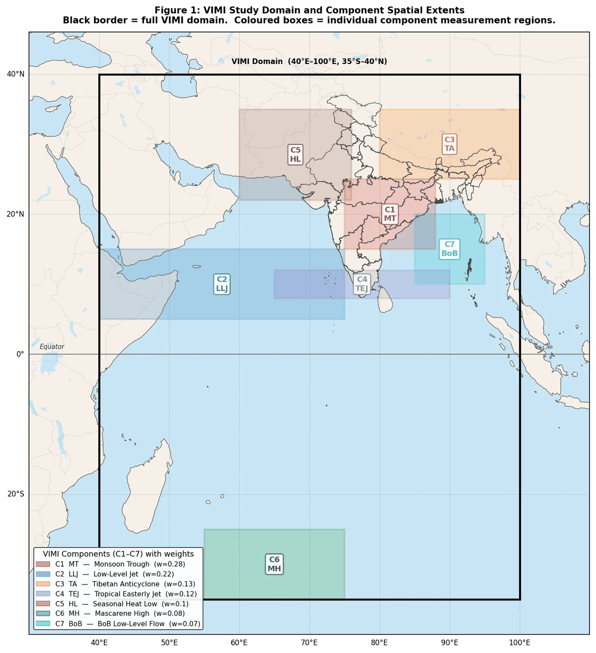
Each component is measured as a cosine-latitude-weighted box mean over a fixed domain, converted to an anomaly against a day-of-year climatology, and normalised to a z-score. Weights are physically motivated by each feature's contribution to Monsoon Core Zone rainfall.
Primary rainmaker. Foothill displacement = break.
Cross-equatorial moisture supply.
Upper-tropospheric exhaust of the heat engine.
Equatorward outflow arm.
Thermal gradient that ignites the circulation.
Southern Hemisphere driver of the LLJ.
Eastern branch — the low-pressure system corridor.
Two of these are not in any existing monsoon index. The Mascarene High is the Southern Hemisphere source of the cross-equatorial jet — every other index measures the jet after it crosses the equator, never its upstream driver. The Bay of Bengal branch is omitted entirely by Arabian-Sea-centric indices, despite being the corridor that delivers monsoon low-pressure systems into central India.
Where the weight sits. The monsoon trough and the Low-Level Jet carry half the index between them (0.50) — the trough because its position determines where rain falls, the jet because it supplies the moisture. These are the two highest-frequency features, and the two that coupled seasonal models represent worst.
3. How the index is computed
zᵢ(t) = [ Fᵢ(t) − Cᵢ(DOY(t)) ] / σᵢ wᵢ — component weight (Σwᵢ = 1.0)
Fᵢ(t) — cosine-latitude-weighted box mean of the component field at time t
Cᵢ(DOY) — climatological long-term mean for the matching day-of-year
σᵢ — anomaly standard deviation
Positive VIMI = active-favourable circulation · Negative VIMI = break-favourable
Derived fields — 850 hPa relative vorticity (C1) and 200 hPa divergence (C3) — are computed by centred finite differences on the native grid before spatial averaging. The climatological baseline is NCEP/NCAR Reanalysis-1 and NCEP/DOE Reanalysis-2 daily long-term means for 1981–2010. Operational runs use NOAA GFS at 0.25° resolution from NOMADS, six-hourly across the full 384-hour range — 65 forecast steps per run.
4. Operational output
Each run produces a 16-day composite time series with the individual component traces overlaid, plus a daily component-attribution panel. The composite answers is the monsoon machinery running? The component panel answers which part of it?
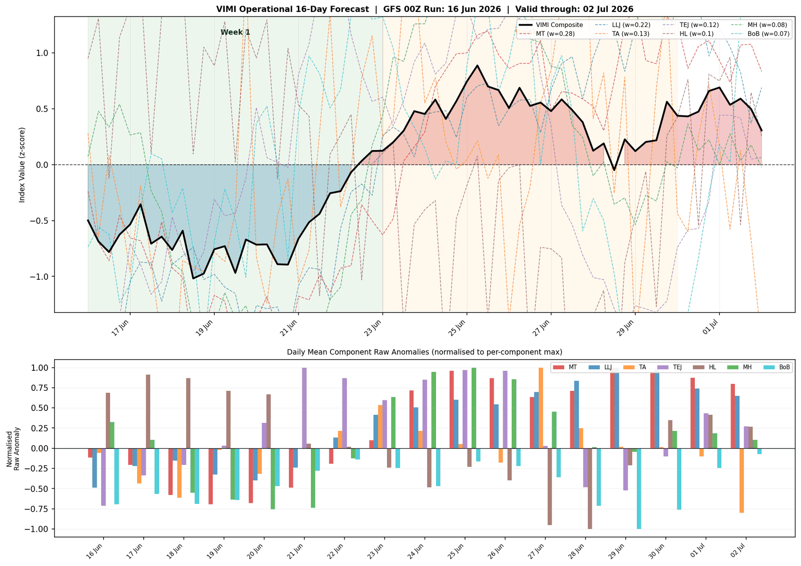
Reading this run. It shows the monsoon suppressed through 21 June — daily mean composite between −0.47 and −0.84 — then crossing zero on 22 June and turning positive from 23 June, staying positive every day through the end of its range on 2 July, peaking at +0.75 on 25 June.
June 2026 finished at −40% of normal, the fifth-lowest June since 1901. The active phase this run projected is the regime that produced the season's first Bay of Bengal low-pressure area on 01–02 July and the first monsoon depression on 04–05 July — the spell that cut the seasonal deficit from −40% on 30 June to −14% by 9 July. This is a single archived run, not a skill statistic, and the index forecasts phase rather than millimetres. But the transition was on the chart at seven to sixteen days' lead.
5. Validation
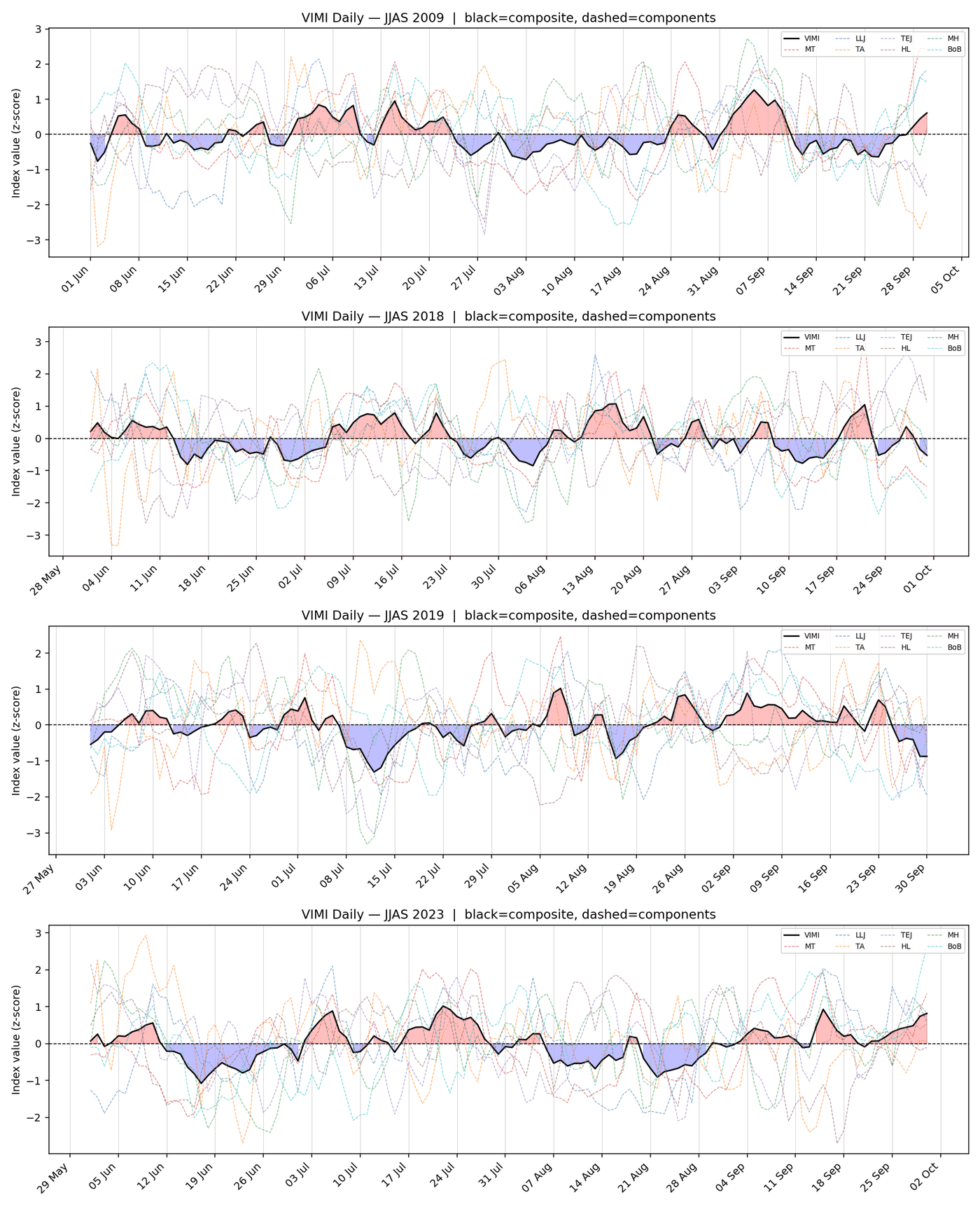
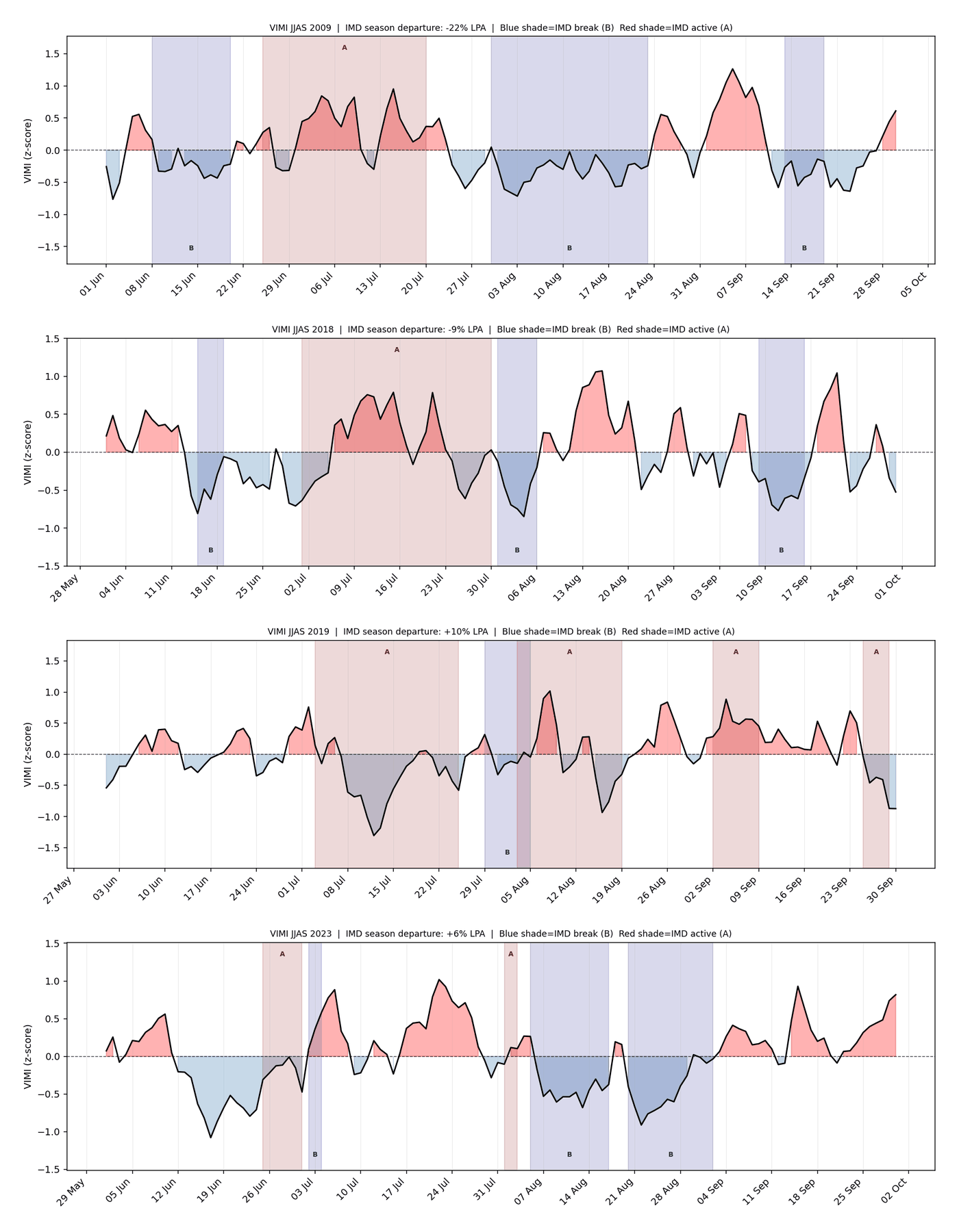
VIMI was computed retrospectively on NCEP/NCAR Reanalysis daily fields for four contrasting JJAS seasons and tested against official IMD Monsoon Season Reports — active and break spell declarations and month-wise rainfall departures. No parameters were tuned to fit.
spell identification
13 of 18 spells
direction accuracy
13 of 16 month-years
2009 · 2018
2019 · 2023
tuned to fit
validation data
| Season | IMD departure | VIMI signature |
|---|---|---|
| 2009 | −22% LPA severe drought |
Predominantly negative across JJAS. Single positive excursion in July, matching IMD's documented exception. Longest negative spell 31 Jul–23 Aug, 24 days. |
| 2018 | −9% LPA below normal |
Balanced signal, active July, suppressed Aug–Sep. All three break spells captured with 0% positive days. |
| 2019 | +10% LPA above normal |
Negative in June (delayed onset, 67% LPA), turning positive into September (77% positive days against 152% LPA rainfall). |
| 2023 | +6% LPA above normal, Aug break |
August break captured at 23% positive days against 64% LPA rainfall. July and September, both +13% LPA, register 74% and 83%. |
The 2009 case
2009 is the most instructive season in the set, because it is the case where a correct seasonal forecast would still have misled you about a specific month. It finished at −22% of LPA, the third most deficient season of 1901–2009. Yet IMD's own end-of-season report records that "all monsoon months except July recorded large deficient rainfall."
positive VIMI days
suppressed
positive VIMI days
ACTIVE
positive VIMI days
deep break
positive VIMI days
suppressed
The index flips clearly positive in exactly the month IMD flags as the exception. And because it is decomposed, it attributes the swing: the Low-Level Jet component moves from a z-score of −0.74 in June to +0.50 in July, its raw anomaly recovering from −3.41 m/s to −0.46 m/s before collapsing back to −2.12 m/s in August. The Somali Jet switched on for a month. Component analysis across the season confirms the LLJ as the most persistently suppressed feature of 2009 — matching IMD's finding that "the cross equatorial flow was weaker than normal during major part of the season."
6. Limitations
This is a version-1 implementation and the constraints are worth stating plainly.
- Self-normalisation. z-scores are currently normalised within each run, which gives a consistent relative scale inside a run but precludes clean cross-run comparison. A climatological σ from a full 1991–2020 daily archive is the fix, and is the priority for v2.
- Fixed bounding boxes. A monsoon trough displaced far south during a strong active spell partly exits its 15–25°N box and reads weaker than it is dynamically. Dynamic feature tracking — following the vorticity and divergence maxima within a wider search domain — is the main methodological upgrade planned.
- TEJ level proxy. The Tropical Easterly Jet is canonically defined at 150 hPa; the current implementation measures it at 200 hPa, introducing a small bias.
- Short spells. Of the five misidentified spells in validation, three were five days or shorter — below the effective resolution of reanalysis box averages — and two fell in an early-season window where self-normalised z-scores rest on a short sample.
- Phase, not rainfall. VIMI forecasts monsoon state — active or break — not millimetres. It is a circulation monitor, not a quantitative precipitation forecast.
Time-varying weights — a heavier Heat Low term in June, a heavier Monsoon Trough term in August — are scientifically motivated by the seasonal evolution of the circulation, but require careful calibration against the full historical archive to avoid overfitting. That work is not done.
7. Read the paper
VayuMet Indian Monsoon Index (VIMI): A Semi-Permanent Feature Based Composite Index for Direct Manifestation of Indian Summer Monsoon Variability
↓ Download PDF Applied to July 2026 →Citation
8. Where this fits
VIMI is not a replacement for seasonal forecasting, and nothing here argues that ENSO-based guidance is wrong. The two operate on different questions.
| Seasonal tier | Intra-seasonal tier | |
|---|---|---|
| Instrument | ENSO · IOD · coupled models | VIMI on GFS |
| Measures | Boundary conditions | The monsoon itself |
| Question | Odds of a below-normal season? | Is the machinery running now? |
| Lead time | Months | 7–16 days |
| Output | A probability category | Active or break, with attribution |
ENSO for the season. Semi-permanent features for the fortnight. Most public monsoon commentary in India runs on the first tier alone — which is why an ordinary intraseasonal swing, like July 2026, gets reported as a broken forecast. The July 2026 case study works through that episode in detail.
Data and references: NCEP/NCAR Reanalysis-1 (Kalnay et al., 1996) · NCEP/DOE Reanalysis-2 (Kanamitsu et al., 2002), daily long-term means 1981–2010, NOAA Physical Sciences Laboratory · NOAA Global Forecast System 0.25° via NOMADS · IMD Southwest Monsoon End of Season Reports 2009, 2018, 2019, 2023 (Met Monograph, Synoptic Meteorology series, National Climate Centre, Pune) · Findlater (1969) · Webster and Yang (1992) · Wang and Fan (1999) · Goswami et al. (1999) · Krishna Kumar et al. (2006) · Rajeevan et al. (2010) · Implemented in Python 3 with xarray, cfgrib, NumPy, pandas, Matplotlib and Cartopy.